Learning MBA Master Degree

TEACHER: Hello, Student! Let me ask you a personal question, please. Did you ever ask an employer for a salary rise?

STUDENT: Yes, a few times. Why?

TEACHER: Did you notice any difference in reactions to your requests according to how the economy was performing at the time?

STUDENT: I see your point. Obviously, it was much easier to get a rise during a boom than during a recession.

TEACHER: Good observation. The prices of all inputs (labor and materials) tend to increase at boom times and to fall during depressions.

STUDENT: Can we say then that "prices of inputs change with the prevalent conditions in the economy"? And I guess this is an important factor to be taken into account in any economic analysis.

TEACHER: The answer to both is yes. As you will recall, when observing the effects of changes in aggregate demand and aggregate demand shocks , for the sake of simplicity we had assumed that input prices did not change.

In a longer term observation we have to study the changes in prices induced by changes in the GDP.

STUDENT: Sounds like a useful approach... but why is it useful?

TEACHER: Because with this more elaborate model we can find out the causes and consequences of the business cycle, and discuss the right fiscal policy measures to stabilize the economy.

Student, you have a good memory. Can you recall how we defined "potential GDP"?

STUDENT: Surely. Potential GDP is the total output possible when all available means of production are employed. And let me add "at their normal rates of utilization".

TEACHER: Very well. You will surely also recall that when the actual output does not coincide with the potential one, we have a GDP (output) gap.

Now let me make a statement on changes in potential output over time.

Over a period of several years, changes in potential GDP may be very important. But over a shorter period (say, 1 year) normally the change is relatively small.

STUDENT: So we will continue to ignore the changes in potential GDP caused by changes in productivity over a one year period.

TEACHER: Right. And since you are so alert today... can you tell me what is the sole element causing variations in the GDP gap if we assume there are no changes in potential GDP?

STUDENT: Yes, I can. The GDP gap will change according to the movements of the actual GDP line around the fixed potential GDP. Nicely pictured in figure B202_1, in Module 2 of this course.

TEACHER: Correct. We will now discuss the effects of changes in input prices

Input Prices and the Output gap

Please take a look at Figure B205_1 below.
Figure B205_1 has two parts, i and ii. In both parts we can see the potential GDP level represented by a vertical line and the SRAS (Short-run aggregate supply) curve. Both are the same in either part of the figure.

In part i the AD (Aggregate demand) curve intersects the SRAS curve at a point below potential GDP. The difference is the "output gap" illustrated by the two-point arrow, in this case a deflationary gap (prices are pushed downwards)

This creates a downward pressure on the price level of inputs; the price level is lower that it would be if the AD curve intersected the SRAS at the equilibrium level (potential GDP).

In part ii the AD (Aggregate demand) curve intersects the SRAS curve at a point above potential GDP. The difference again is the "output gap" illustrated by the two-point arrow, but in this case it is an inflationary gap.

This creates an upward pressure on the price level of inputs; the price level is higher that it would be if the AD curve intersected the SRAS at the equilibrium level (potential GDP).

STUDENT: OK, let me see. The output gap is a good indication of the pressure of demand on input prices.

If GDP is higher than potential output, demand for input will be high, and vice-versa. In other words, when we see an inflationary gap actual output exceeds potential and there will be an upward pressure on input prices. And vice-versa, of course.

But I have a question, does this affect all inputs?

TEACHER: The relationship is true for all inputs. But the degree of pressure may change according to the availability of each input. Labor for instance is usually an input whose total availability can not change rapidly, and once it is fully employed it is hard to get additional supply.

Let’s discuss the effect of the GDP gaps on wages (labor costs).

The effect on wages depends very much on the legal environment and the relative forces of labor unions. In the US there is little legal restraint on firing people or reducing wages; as for unions, there are great differences between industries. In many European countries on the other hand there are important legal restraints on firing and wage reduction.

There is no truly "right" answer to the question of which of these situations is better. Obviously the US economy is much more flexible in responding to changes in the output gap and thus the return to the equilibrium level is quicker than in most European countries. After a time most people are better of as the GDP returns to the equilibrium level. But it is also true that in the European system there is less human suffering in the short run.

STUDENT: And what about firm’s profits?

TEACHER: Naturally profits tend to diminish during a deflationary gap and to increase during an inflationary gap, a "boom".

But returning to wages, it is a fact that in industrial economies labor costs tend to grow more rapidly during a boom than they fall during a recession. Again this is due mostly to legal or union enforced impediments to reduce wages.

STUDENT: This is true, because people resist reductions in nominal wages. If a worker earns $5 and hour he will strongly resist getting paid $4, and the government and the unions will usually support him. But I have noticed that there is a lot less resistance to reductions in real wages. Our worker may not resist as much or get the same support from government and unions if he gets the same $5 an hour but due to the inflationary pressure on prices his purchasing power is reduced by 20%.

TEACHER: Very true, and reducing real wages via inflation and eventual devaluation of the currency is common, because it is politically easier to attain that reducing nominal wages and avoiding inflation.

The long-run effects of aggregate demand shocks

Expansionary shocks

Let’s imagine that we are on an almost ideal situation; the economy is operating at a stable price level at full employment, as we can see represented in Figure B205_2 part i, when the Aggregate Demand curve is AD1.
Now something happens to disturb this idyllic picture; we can imagine that there is a sudden and sizable increase in autonomous demand due to say a boom in investment spending.

In the same part i of the figure we see the first effect of this change.

The Aggregate Demand curve is now AD2 . Starting from full employment, the AD curve shifts upwards along a given SRAS curve. There is an increase in GDP, and as output expands beyond its normal capacity, there is pressure on the input price level and prices go up.

In part ii of the figure we see the next effect, delayed in respect to the previous one: as prices of inputs go up, the SRAS curve shifts upwards. Prices are higher at every level of output.

Notice that the shift of the SRAS curve causes GDP to fall along the AD curve. This process does not stop until actual output falls back to its potential level, but now at a higher price level.

STUDENT: Your explanation shows that a one time expansionary shock, starting from full employment, causes an inflationary shock. And eventually actual GDP is equal to potential again, at a higher price level. I also interpret that trying to get more output and income from a full employment economy via an increase in expenditure is possible only for a short time, and with the consequence of creating inflation.

TEACHER: Almost completely correct. And I say "almost" because we must distinguish between the one-time increase in prices created by a one-time increase in expenditure, and spiraling inflation.

In the case we are discussing, you can see in part ii of the figure that once the economy has returned to its potential output, the inflationary gap disappears. There is no more inflation. There is an "automatic" adjustment mechanism that over time eliminates the inflationary pressure, and prices stabilize... but at a higher level than before.

STUDENT: I guess we can summarize by saying that increasing expenditure when actual GDP is below potential may produce a sustainable increase in output at stable prices. The same increase in expenditure under full employment only produces a temporary increase in output that soon returns to equilibrium level at a higher price level.

TEACHER: True. The only way to increase output permanently over and above the full employment level is to increase productivity.

STUDENT: Sure. If we start from full employment and for some reason we begin to obtain more output out of the same labor force, this gain in productivity will mean that potential GDP increases. But this is normally a slow process, right?

TEACHER: Relatively slow, yes. Historically we can observe periods of almost no gain in productivity in industrial economies, contrasting with improvements of the order of 3 to 4% a year in other periods.

Deflationary shocks

Starting again from the ideal position of full employment at equilibrium GDP we will now discuss the results of a sudden fall in autonomous expenditure, such as a reduction in investment or exports.

For this analysis we will have to distinguish between a flexible and inflexible wage environment. Let’s begin with a flexible wage situation first.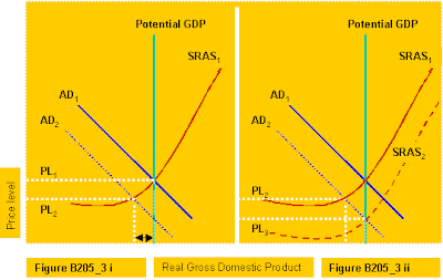
Figure B205_3 has two parts. Part i is similar to Figure B205_2, because we start from the same equilibrium situation. As the AD curve shifts downwards from AD1 to AD2 , price level falls as well as actual GDP, and a recessionary gap opens. Slowly the SRDS curve, responding to the fall in input prices and wages, shifts rightwards, as shown in part ii of the figure. Eventually the recessionary gap closes, and the actual GDP is again at equilibrium but at a lower price level that when the fall in AD started.
STUDENT: This seems to be again an automatic stabilization process at work. But of course it means lower wages and a lower standard of living for workers. And what happens if due to government and/or labor union pressures wages do not fall?

TEACHER: In this case the economy will stay in the position shown in part i of the figure for an indefinite time. There will be unemployment but the workers who keep their jobs will earn the same as before. From a social point of view, societies have to make a difficult decision. Which is better, return to full employment at lower wages, or maintain the level of wages for some workers while others have no jobs?

Anyway, wages are "sticky" not only due to government and/or labor union pressures. Employers are also reluctant to reduce wages because they are afraid of de-motivating efficient employees, and of other consequences such as getting a reputation of ruthlessness.

In any case, the rightwards shifting of the SRAS is normally slow and not sufficient to close the deflationary gap. Normally, if the economy is to return to a situation of equilibrium (actual equal to potential output), it becomes necessary to shift the AD upwards.

STUDENT: Nice. No one would suffer. We go back to full employment at the previous level of wages. But easier said than done, I presume.

TEACHER: Let’s discuss this question in the following paragraph.

Fiscal Policy and the Business Cycle

As you know, macro was developed not just to explain the business cycle but mainly to find solutions to avoid or at least minimize fluctuations and the consequent human suffering during depressions. Keynes and his followers argued that fiscal policy was the tool to use to achieve counter-cyclical effects. Later on macro included monetary policy as an effective counter-cyclical element. But we will discuss monetary policy later on. Presently we will concentrate on fiscal policy.

Discretionary Fiscal Policy

This is the name given to fiscal policy when changes in tax rates and government expenditure are made deliberately with the purpose of stabilizing the economy as close as possible to full employment at equilibrium GDP level.

We have already mentioned that determining the direction of changes in fiscal expenditure and taxes is not difficult. Do you remember, Student?

STUDENT: Of course. In a recession government must increase spending and or reduce taxes, and vice-versa. These measures cause a shift of the AD curve in the desired direction.

TEACHER: Correct. The problem consists in determining when and how much to change tax rates and expenditure; that is, in determining the right moment and the right amount of the changes to be made in the mentioned variables. It is easy to err on either side: to soon, too late, too much, or too little fiscal policy actions.

But anyway it is better to have a counter-cyclical tool, no matter how imperfect, than not having any tool as was the case before Keynes.

Let me finish this Module by mentioning the paradox of thrift. We have already discussed the fallacy of composition, of which the paradox of thrift is a special case. But may be you can take over from here, Student.

STUDENT: Sure. A classical example of the fallacy of composition is the case of a short person sitting in a theater. If this person stands up, he or she will see much better. But if everyone else in the theater stands up, the short person is worst off than before.

Applied to saving vs. spending decisions, saving may be good for individuals or firms as long as few of them do it. But if a sizable proportion of firms and individuals increase savings, our "famous" AD curve will shift downwards and to the left, opening a deflationary gap... and everyone will be worst off than before.

TEACHER: Very well. And this is the end of Module V. See you later!